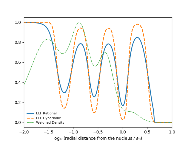
EX4: ELF rational vs. hyperbolic transformation

Compute ELF and visualize spherically averaged ELF for Kr atom using ‘rational’ & ‘hyperbolic’ transformations.

import numpy as np
import matplotlib.pyplot as plt

from chemtools import Molecule, ELF
from horton import AtomicGrid

# 1. Build Molecule, AtomicGrid and ELF model

mol = Molecule.from_file('atom_kr.fchk')
grid = AtomicGrid(mol.numbers[0], mol.pseudo_numbers[0], mol.coordinates[0],
                  agspec='exp:0.005:10.0:200:194', random_rotate=False)

elf_r = ELF.from_molecule(mol, grid=grid, trans='rational', trans_k=2, trans_a=1)
elf_h = ELF.from_molecule(mol, grid=grid, trans='hyperbolic', trans_k=1, trans_a=1)

# 2. Compute spherically-averaged density ($4.0 \pi r^2 \rho$) & ELF

elf_r = grid.get_spherical_average(elf_r.value)
elf_h = grid.get_spherical_average(elf_h.value)
dens = grid.get_spherical_average(mol.compute_density(points=grid.points))
dens *= (4.0 * np.pi * grid.rgrid.radii**2)

# 3. Plot ElF and (scaled) radially weighted density versus radius

logx = np.log10(grid.rgrid.radii)
plt.plot(logx, elf_r, linewidth=2, linestyle='-', label='ELF Rational')
plt.plot(logx, elf_h, linewidth=2, linestyle='--',  label='ELF Hyperbolic')
plt.plot(logx, 0.01875 * dens, linestyle='-.', linewidth=1, label='Weighed Density')
plt.legend(loc='lower left', fontsize=8, frameon=False)
plt.xlim(-2., 1.)
plt.xlabel('log$_{10}$(radial distance from the nucleus / $a_0$)')
plt.show()

Total running time of the script: ( 0 minutes 1.003 seconds)