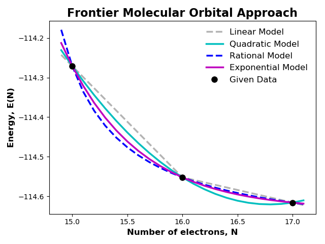
EX8: Plot Energy Models (Frontier MO)

Compute linear, quadratic, rational and exponential energy models for various number of electrons using frontier molecular orbital (FMO) approach and plotting E vs. N.

import numpy as np
import matplotlib.pyplot as plt
from chemtools import GlobalConceptualDFT

# 1. Build linear and quadratic energy models using FMO approach

# path to molecule's fchk file
file_path = 'ch2o_q+0.fchk'
# build linear & quadratic global conceptual DFT tool (one file is passed, so FMO approach is taken)
model_lin = GlobalConceptualDFT.from_file(file_path, 'linear')
model_qua = GlobalConceptualDFT.from_file(file_path, 'quadratic')
model_rat = GlobalConceptualDFT.from_file(file_path, 'rational')
model_exp = GlobalConceptualDFT.from_file(file_path, 'exponential')

# 2. Compute energy values for various number of electrons.

# get reference number of electrons, n0, from either linear or quadratic models
n0 = model_lin.n0
# sample number of electrons around n0
n_values = np.arange(n0 - 1.1, n0 + 1.1, 0.1)
# compute linear & quadratic energy values for sampled number of electrons
energy_lin = [model_lin.energy(n) for n in n_values]
energy_qua = [model_qua.energy(n) for n in n_values]
energy_rat = [model_rat.energy(n) for n in n_values]
energy_exp = [model_exp.energy(n) for n in n_values]

# 3. Plot energy vs. number of electrons.

# plot linear energy model
plt.plot(n_values, energy_lin, color='0.7', linestyle='--', linewidth=2.5,
         label='%s Model' % model_lin.model.capitalize())
# plot quadratic energy model
plt.plot(n_values, energy_qua, color='c', linestyle='-', linewidth=2.5,
         label='%s Model' % model_qua.model.capitalize())
# plot rational energy model
plt.plot(n_values, energy_rat, color='b', linestyle='--', linewidth=2.5,
         label='%s Model' % model_rat.model.capitalize())
# plot exponential energy model
plt.plot(n_values, energy_exp, color='m', linestyle='-', linewidth=2.5,
         label='%s Model' % model_exp.model.capitalize())

# 4. Plot data points used for modeling energy.

# number of electrons used for modeling energy
n_data = [n0 - 1, n0, n0 + 1]
# compute energy values used for modeling energy
# Note: any of the tools built above can be used for this purpose because
#       they all have the same energy for N0 - 1, N0, and N0 + 1 electrons.
e_data = [model_lin.energy(n) for n in n_data]

# plot given data points
plt.plot(n_data, e_data, marker='o', markersize=8, color='k', linestyle='', label='Given Data')

# add axis label
plt.xlabel('Number of electrons, N', fontsize=12, fontweight='bold')
plt.ylabel('Energy, E(N)', fontsize=12, fontweight='bold')
# add title
plt.title('Frontier Molecular Orbital Approach', fontsize=16, fontweight='bold')
# add legend & remove legend frame
plt.legend(frameon=False, fontsize=12)
# show plot
plt.tight_layout()
plt.show()

Total running time of the script: ( 0 minutes 0.592 seconds)