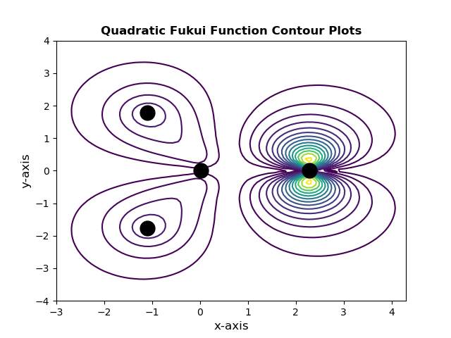
EX10: 2D-Contours Quadratic Fukui Function (FMO Approach)

1. Make a 2D grid in the plane containing formaldehyde, \(\mathbf{CH_2O}\).
2. Build a quadratic energy models using frontier molecular orbital (FMO) theory approach.
3. Evaluate quadratic Fukui function on the grid points.
4. Plot 2D-contour plots of quadratic Fukui function.

import numpy as np
import matplotlib.pyplot as plt
from chemtools import LocalConceptualDFT, mesh_plane


# 1. Make a 2D grid in xy-plane (molecular plane).

xyz = mesh_plane(
    np.array(
        [
            [2.27823914e00, 4.13899085e-07, 3.12033662e-07],
            [1.01154892e-02, 1.09802629e-07, -6.99333116e-07],
            [-1.09577141e00, 1.77311416e00, 1.42544321e-07],
        ]
    ),
    0.1,
    6,
)

# 2. Build a quadratic energy models using FMO approach

# path to molecule's fchk file
file_path = "ch2o_q+0.fchk"
# build a quadratic global conceptual DFT tool
tool = LocalConceptualDFT.from_file(
    file_path, model="quadratic", points=xyz.reshape(-1, 3)
)

# 3. Evaluate quadratic Fukui function on the grid points.

ff_quad = tool.fukui_function.reshape(xyz.shape[:2])

# 4. Plot 2D-contour plots of quadratic Fukui function.

# sample contour lines
levels = np.array([0.001 * n * n for n in range(500)])
# plot contours of quadratic Fukui function
plt.contour(xyz[:, :, 0], xyz[:, :, 1], ff_quad, levels)

# plot atomic centers
x_atoms, y_atoms = tool.coordinates[:, 0], tool.coordinates[:, 1]
plt.plot(x_atoms, y_atoms, marker="o", linestyle="", markersize=15, color="k")

# setting axis range & title
plt.axis([-3.0, 4.3, -4.0, 4.0])
plt.title("Quadratic Fukui Function Contour Plots", fontweight="bold")
# add axis label
plt.xlabel("x-axis", fontsize=12)
plt.ylabel("y-axis", fontsize=12)
# show plot
plt.show()

Total running time of the script: ( 0 minutes 0.638 seconds)